Time History Analysis of Steel U-Girder Bridge

Please fill out the Download Section (Click here) below the Comment Section to download the Full Webinar PDF File 

The fatigue analysis is one of the assessment methods of bridges. Time History Analysis can be used to calculate the fatigue stresses. In this course, we tried to broaden your understanding of functions that are for time history analysis in midas Civil. In addition, we walked through in detail the process of time history analysis. It will be helpful to most of the bridge engineers who handle the time history analysis.

This 1-hour course covers the full process, from setting up options for the time history analysis to checking results. The actual steel U-bridge model from a real project was used in the training. 

This Project Tutorial highlights:

1. What to do to consider dynamic behavior of the bridge

In the dynamic analysis, not only the magnitude of loads but also the speed of loading or the frequency of loading affects the results. Therefore, we determine the mode of structure and check the dynamic response of the structure. 

2. How to define the time history analysis data

We will follow three steps to define the time history analysis data.

1) Time Forcing Functions

2) Time History Load Cases

3) Dynamic Nodal Loads

3. How to check results from Time History Analysis

midas Civil provides a lot of useful functions to verify the results from the time history analysis. We will follow several steps to get the stress and deformations along time.

1. What to do to consider dynamic behavior of the bridge

The eigenvalue analysis is necessary for all of dynamic analysis. Through the eigenvalue analysis, we can obtain the eigenvalue and eigenvector of structures. We can predict the dynamic behavior of the bridge using the eigenvalue and eigenvector. For instance, in the perspective of the whole bridge, the eigenvalue could be displacement and the eigenvector could be frequency. If the eigenvalue analysis is conducted for the column, the eigenvalue could be the buckling load and the eigenvector could be the buckling shape.

In order to perform the eigenvalue analysis, we need the mass of structures. midas Civil provides functions to convert structure bodies or dead loads to masses for the eigenvalue analysis.

Loads to Masses function

This function converts static load cases to masses. The process is simple.

1. Select the direction of mass

2. Select load types

3. Set the gravity acceleration

4. Select load cases

5. Input a scale factor

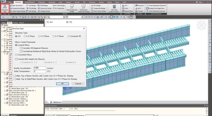
Convert Self-weight into Masses option in Structure Type function

This option converts structures to masses. If this option is used, elements that have material properties will be converted to masses automatically. If the self-weight is considered as beam element loads or pressure loads and etc, this option should be checked off to avoid to take masses of self-weight double. 

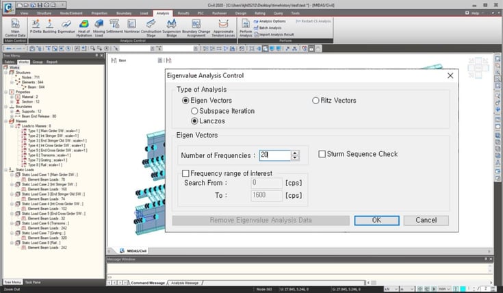
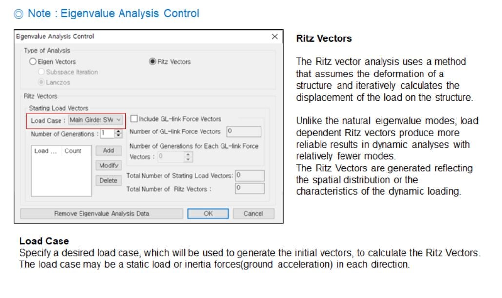
Lastly, we need to use Eigenvalue Analysis Control function(Analysis tab > Eigenvalue function). Here you can input the number of frequencies and select the type of analysis.

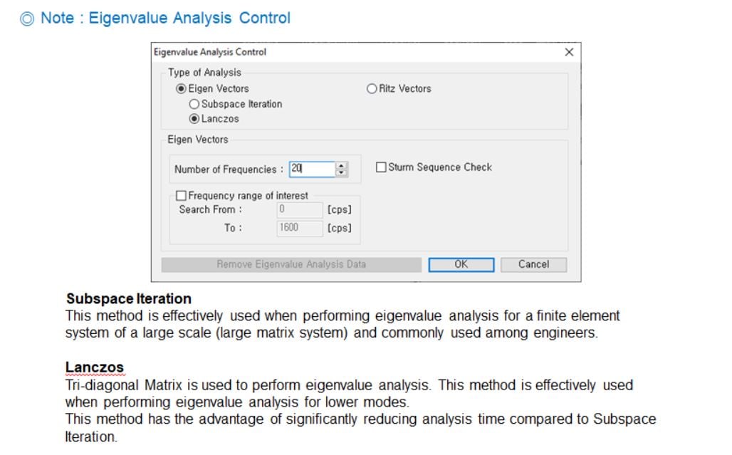
The type of analysis has the feature as shown below.

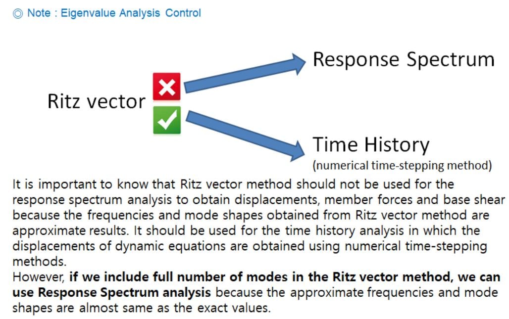
To check that converted masses are properly used for the eigenvalue analysis, compare two values.

1. Total reaction results for self-weight and additional dead loads / the gravity acceleration

2. Accumulated modal masses of the higher mode / the ratio of modal participation masses

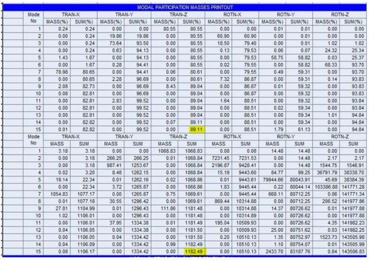
For instance, let's take a look at the figures below. These show reaction results and modal participation masses.

- A, Total reactions: 13,182 kN

- B, The gravity acceleration: 9.81 m/s2

- A', The ratio of participation: 89.11 %

- B', Accumulated masses: 1,183 ton

A/B  = 13,182/9.81 = 1,343 ton

A'/B' =1,183/0.8911 = 1,327 ton

A/B and A'/B' show similar values therefore, we can guess that mass data is used for the eigenvalue analysis properly in this example model.

2. How to define the time history analysis data

Now, we take 3 steps to perform the time history analysis in midas Civil. 

A. Time History Function

B. Time History Load Cases

C. Dynamic Nodal Loads

A. Time History Function

Here, we define a function about the relationship between one item among 5 items(Normalized acceleration, Acceleration, Force, Moment, and Normal) and time. 

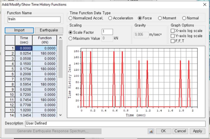
If there is train load data, we can define a load function for the time history function. The function is Train Load Data Generator in Tools menu. We can import the load data to the time history function simply. 

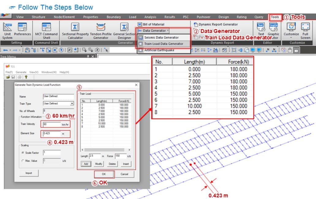
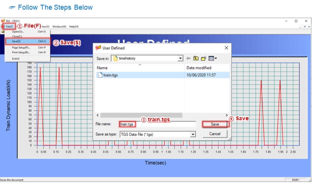
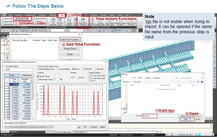
B. Time History Load Cases

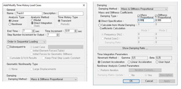
After defining the time history function, move onto Time History Load Cases function. We can select the type of analysis, the analysis time, the increment of time, damping ratio, and etc.. in the time history load cases function.

C. Dynamic Nodal Loads

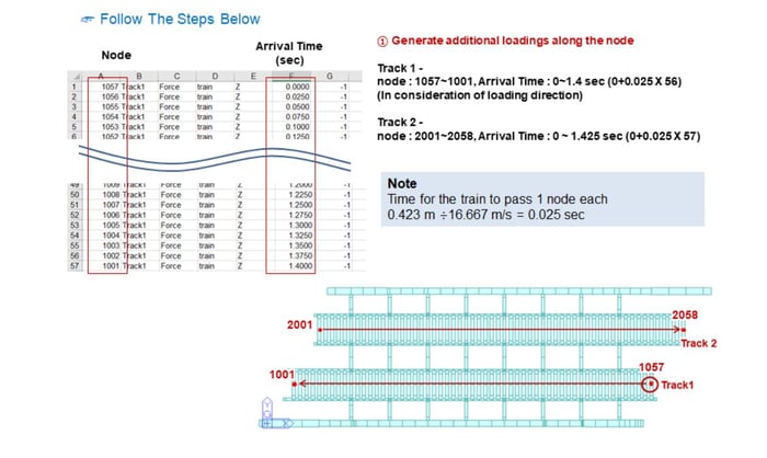
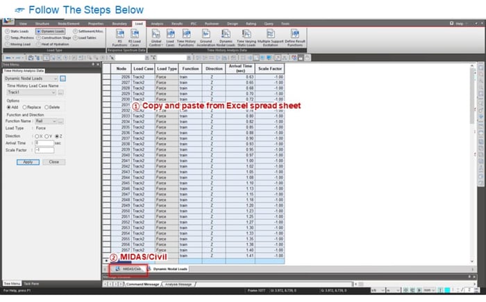
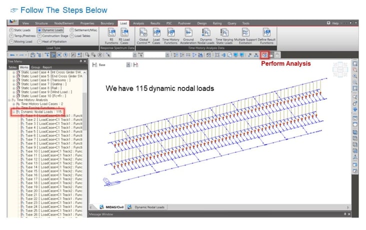
This is the last step for the preparation of the time history analysis. In Dynamic Nodal Loads function, we will assign each time history function to a node of elements and time-history load cases. We need to set different arrival times to consider the movement of a train load. We can calculate the arrival times using the formula below.

The arrival time = Distance from the starting point to a desired node / the velocity of the train

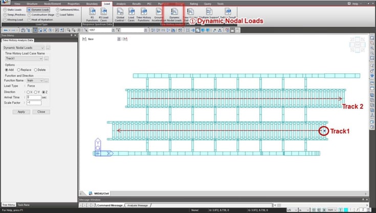
It is time-consuming work to define the dynamic nodal load to each node. We would recommend you to organize the number of nodes and to use a spreadsheet.

3. How to check results from Time History Analysis

After the time history analysis, we can check results in various views. We had the eigenvalue analysis. The results of the eigenvalue analysis is shown in Vibration Mode Shape. 

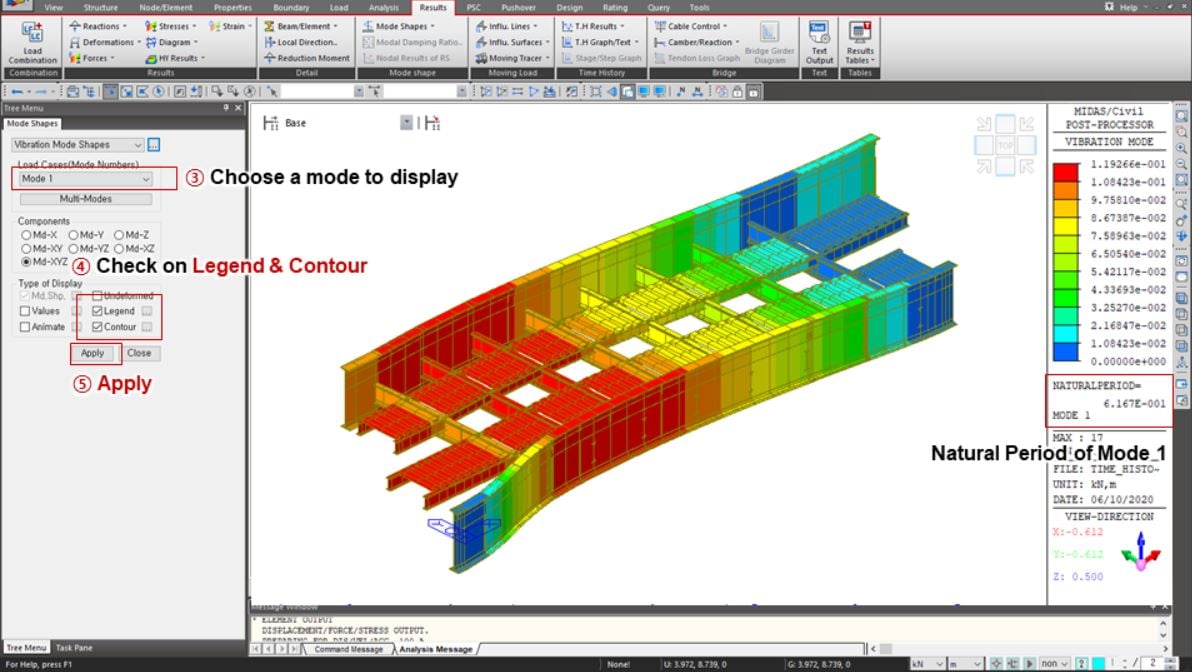
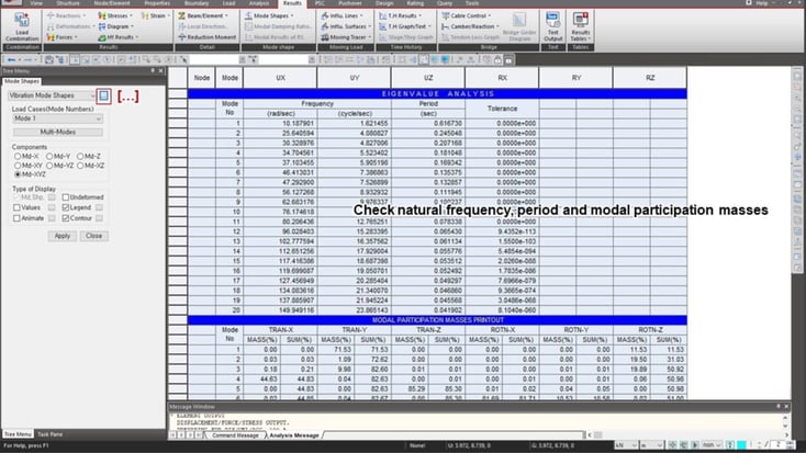
The results of the time history analysis can be checked in Results view.

Here, we can check envelop results.

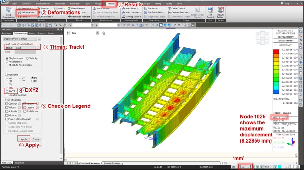
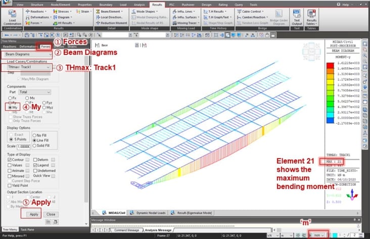
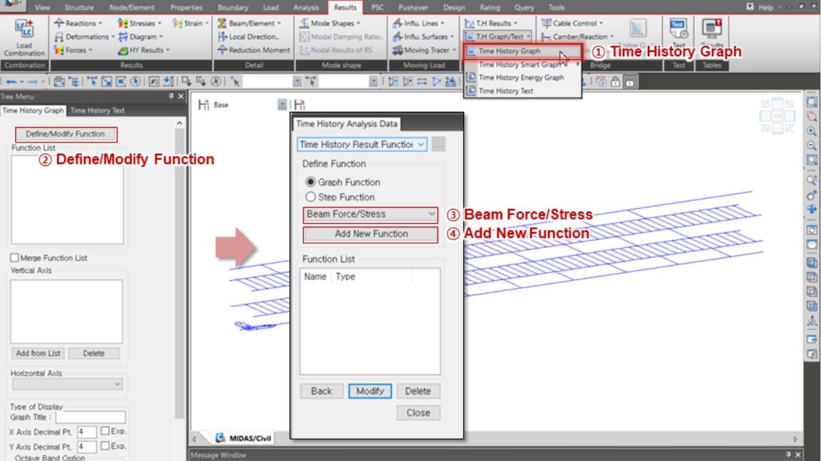
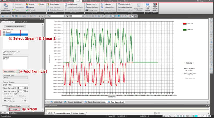
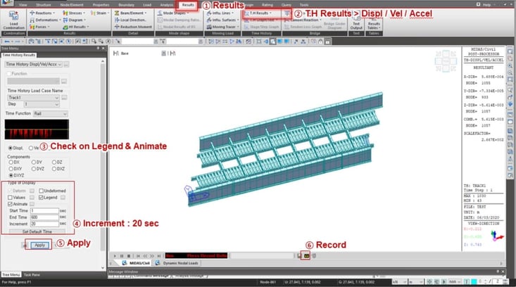
The results of time history analysis can be obtained as the graphical format or text format. And also the results can be shown in the model view along the time history. You can find related functions in Time History Results under Results tab.

Watch the full webinar video